Shared news
Expectations can change together
News about inflation or growth can change expected policy paths in several economies at once. US and Swedish yields may then rise together even without a distinct US shock causing the Swedish move.
Buying a home in Sweden, I want to understand what could change my monthly mortgage payment—and what I would get by paying to fix the rate. News about US bond yields feels distant. An extra few thousand kronor a month does not.
On a SEK 5 million mortgage, a rise from 3% to 4% adds about SEK 4,167 a month in gross interest. To judge whether a fixed offer is worth its price, it helps to follow the route from market rates to the bank’s quote, then test the offers against a budget you could keep paying.
A mortgage is a loan from a bank to a household. A bond is a loan that investors can buy and sell. In both cases, the lender commits money now for payments later. The interest rate depends on when those payments arrive, how certain they are and what else the lender could do with the money.
A bond’s yield is the return implied by its price and promised payments. When investors demand a higher return for the same payments, the price falls and the yield rises. An outstanding fixed coupon does not change. A borrower issuing a new bond then faces the higher market cost.
An investor can buy a five-year bond or keep reinvesting in short-term instruments. If expected short rates rise, the long bond must compete with that better expected alternative. The comparison covers the expected path of short rates over all five years. Long yields can therefore rise while today’s central-bank rate stays still. Federal Reserve: the yield curve and expectations
The policy rate anchors the shortest rates in a currency. Inflation and growth news change expectations about where policy will go. The term premium can change separately: investors may demand more compensation to hold long bonds when the outlook is uncertain or more bonds need buyers. Strong demand for safe assets can lower the premium, sometimes below zero. Central-bank bond purchases can also affect it by changing the supply available to other investors. Riksbank: expectations, term premia and bond supply
The term premium concerns the risk of holding a long interest-rate position. A bank bond also exposes its owner to the issuer and to the ease of selling the bond. Compensation for those credit and liquidity risks can move independently of the underlying interest-rate curve. During a market scare, safe government yields can fall while banks’ borrowing premiums rise. Riksbank: funding costs during stress
To price a mortgage, the bank combines its funding costs with the cost of running the loan, holding capital and covering expected losses. Competition and the borrower’s terms affect the quote too. A bond yield captures only part of that price. Riksbank: the funding mix and retail pricing
Pension funds, insurers, banks and asset managers hold bonds in several countries. They react to shared news and compare returns across markets. A change in the return they require in one country can alter the prices they accept in another, even when national central banks set different policy rates.
News about inflation or growth can change expected policy paths in several economies at once. US and Swedish yields may then rise together even without a distinct US shock causing the Swedish move.
If a foreign bond becomes more attractive after currency hedging and risk, investors may shift demand toward it. Other bonds may need lower prices and higher yields to compete. Intermediaries’ funding and risk limits can transmit changes too.
Kearns, Schrimpf and Xia study announcements from seven central banks and yields in 47 recipient economies, including Sweden. They find stronger spillovers at long maturities and a stronger relationship with financial openness than with trade links. That provides evidence for a financial connection beyond simple same-month correlation. The estimates remain conditional on their shock definitions. International spillover study, sections 2 and 6
A Swedish investor who owns a dollar asset also faces the dollar–krona exchange rate. Hedging locks in a future conversion rate. The forward price normally offsets the interest differential between comparable investments over the hedge’s maturity. Costs and a cross-currency basis, the gap between direct and currency-swapped financing costs, can alter the comparison. A three-month currency hedge does not lock in hedging costs for the full life of a ten-year bond. Raw US and Swedish yields therefore need not become equal. BIS: currency hedging and the cross-currency basis
The connection also runs through banks’ own borrowing. The BIS describes Swedish mortgage banks obtaining foreign currency and swapping it into kronor, alongside domestic institutional investors hedging foreign assets in the opposite direction. Changes in these hedging demands or dealers’ capacity can affect the cost of Swedish funding. BIS, the Swedish example on pp. 55–56
Sweden has had a floating exchange rate since 1992. The Riksbank can choose its short policy rate while the currency, expectations of future policy and longer-term risk premia adjust. Sweden can therefore set its own policy rate while longer market yields respond to news abroad. Riksbank: the move to a floating krona · Evidence on short- versus long-rate spillovers
A global term-premium rise can pull Swedish long yields higher while the Riksbank holds its rate unchanged. A broader inflation shock can also change Sweden’s expected policy path. A funding scare can raise bank spreads even as government yields fall. The origin of the move determines which component reaches a mortgage.
A bank lends to a household for many years while its own funding costs can change. It uses funding and hedges to manage that exposure. Four market prices help explain the cost.
Government bonds and swaps are different benchmarks. The relevant comparison matches currency and maturity; a government yield is a useful public proxy rather than the bank’s exact hedge price. Riksbank funding framework, pp. 4–7
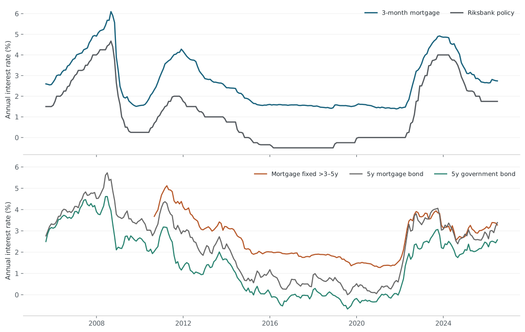
Consider the 2013 taper period. From April to September, US ten-year yields rose 107 bp, Swedish five-year government yields rose 74 bp, and Swedish mortgage rates fixed for over three to five years rose 31 bp. The Riksbank rate stayed at 1%; floating mortgage rates fell 18 bp. These are changes between monthly averages, calculated from the downloaded data.
An observed sequence of related prices, not an isolated US shock experiment. The month endpoints are selected to illustrate different exposures; other news and bank decisions also occurred.
For a newly fixed loan, the bank wants funding and hedging costs aligned with its promised interest receipts. If the matched-maturity SEK swap rate rises and its funding premium stays unchanged, a comparable new loan costs more to fund. That creates pressure on the fixed mortgage quote.
For a floating loan, the bank can issue that fixed-rate bond, receive a fixed rate through a swap, and pay three-month STIBOR. The received fixed leg offsets most of the fixed bond payment. What remains is a floating reference rate plus the bond–swap premium. A general rise in both long bond and swap rates need not raise this net floating cost by the same amount. Riksbank: converting fixed funding into floating costs
Dollar funding also has to be converted into kronor. The dollar borrowing cost and FX-swap cost belong in the same calculation. Their combined effect can move STIBOR relative to expected Riksbank rates. Adding an unhedged US Treasury rate to Swedish funding costs would misrepresent this mechanism. Sveriges Riksbank, Fact box on STIBOR transmission, pp. 19–20
Deposits and other borrowing change the bank’s average cost. Operating expenses, capital requirements, expected losses and commercial pricing then affect the mortgage quote. Slower repricing of deposits can damp policy pass-through; competition or a change in the bank’s desired markup can change it further. Riksbank: deposits and mortgage-rate pass-through
The 2024 Riksbank framework makes the role of deposits explicit, holding its other components constant.
Its December 2023 sample had roughly 51% deposits, 41% covered bonds and 8% other funding. These are sample-specific historical weights. Peter Kaplan and Mambuna Njie, Riksbank, 22 May 2024
Published studies find that three-month mortgage rates respond strongly to Swedish policy and short-term funding costs. Longer fixed offers are more exposed to borrowing and hedging costs over several years. How much reaches borrowers depends on the episode and whether the study measures advertised rates or the rates people actually pay.
Kaplan and Njie’s 2024 Riksbank study follows actual mortgage rates across policy cycles. During the tightening from March 2022 to October 2023, floating mortgage rates rose by about 80 basis points for each 100 basis points of policy-rate increase. The corresponding average in the earlier cycles was about 92. Deposits, other funding costs and bank pricing help explain the difference. These figures compare whole cycles; the adjustment at a particular reset date can differ. Kaplan and Njie, 2024
The Riksbank’s covered-bond purchases provide a more direct test of the funding channel. In a study of the purchase announcements, a 10 basis-point fall in covered-bond yields was followed by an estimated 10 basis-point fall in one-to-two-year fixed mortgages, compared with about 2 basis points in floating mortgages. The estimate supports stronger fixed-rate exposure to longer funding costs, but it comes from only eight announcements. It disappears when three major pandemic announcements are omitted. Emanuelsson, Andersson and Vasi, 2022
The May 2026 Financial Stability Report describes a related episode. STIBOR and longer funding costs rose while the policy rate stayed unchanged, and banks raised both floating and fixed mortgage rates. An unchanged Riksbank rate therefore leaves room for a mortgage offer to become more expensive. Riksbank Financial Stability Report 2026:1
The international study introduced earlier separates news about today’s policy rate, the future policy path and longer-term yields. A daily change in the US ten-year yield combines these influences. Its effect on Swedish financing therefore depends on what caused the move. Kearns, Schrimpf and Xia, 2019
Swedish research reaches a compatible conclusion. Both US and German rates help explain Swedish yields, but they contain overlapping information. In one Riksbank specification, the US coefficient even changes sign when Germany and financial stress are included. That instability makes European and Swedish prices essential to interpreting the US move. The negative coefficient alone cannot establish that higher US yields reduce Swedish borrowing costs. Riksbank term-premium study, 2023 · Finansinspektionen swap-rate decomposition, 2019
Narrow announcement-window studies try to isolate news by measuring market surprises around a known event. That is stronger than regressing monthly yields on each other. Identification still depends on what else the announcement reveals, market liquidity and how the shock is scaled. The international study separates target, policy-path and long-yield residual shocks; a raw US ten-year change combines all three plus other news. Jonathan Kearns, Andreas Schrimpf and Fan Dora Xia, RBA RDP 2019-03, April 2019
Controlling for Germany can remove both common global news and part of a genuine route from the US through Europe. Controlling for Sweden’s own curve can remove a further transmission channel. A small conditional US coefficient cannot establish that the total US influence is small.
For this analysis, I use SCB’s monthly rates on new and renegotiated mortgages from monetary financial institutions (MFI), alongside daily market series distributed by the Riksbank. Floating-rate history spans September 2005–July 2026, 251 months. The detailed fixed-rate bins begin in September 2010, giving 191 months. Market observations are averaged within each month; September 2026 is excluded from estimation. SCB dataset · Riksbank series
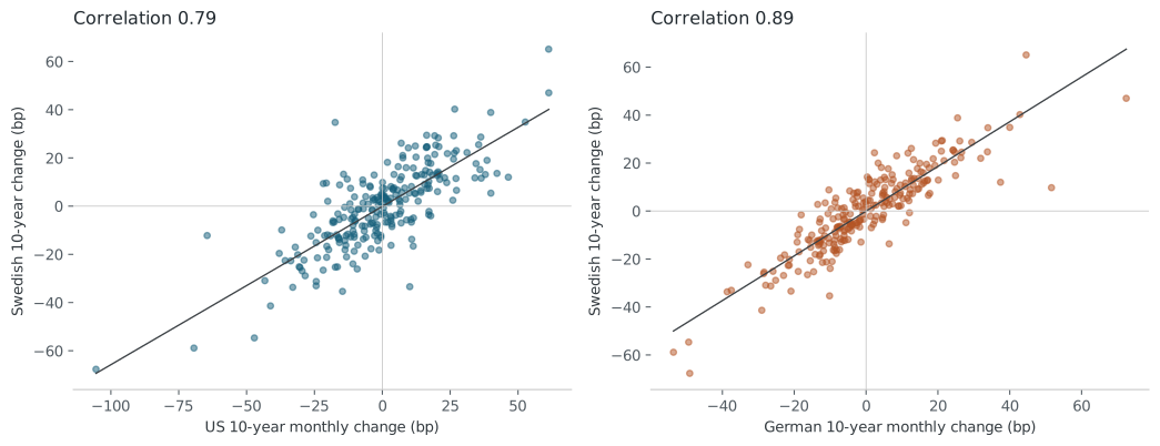
US and Swedish ten-year yields often move in the same direction. Across 250 monthly changes, their correlation is 0.79, where 1 would mean perfectly aligned movements. A model using only US yields associates a one percentage-point US increase with a 0.66 percentage-point Swedish increase. The chart lets you see the monthly observations behind that estimate.
Germany changes the interpretation. Once the model also accounts for German yields, the estimated US association falls to 0.19 percentage points. Much of the original relationship is shared with Europe. Some of that can be common news; some can be transmission from the US through European markets. The adjustment cannot distinguish those explanations, so the smaller coefficient is not an estimate of America’s total influence.
Each coefficient below describes the Swedish ten-year yield change associated with a 1 percentage-point change in the named foreign yield. Parentheses give 95% confidence limits for the estimate. The fit column describes historical variation explained by the model; it does not measure forecasting accuracy.
| Swedish 10y model | US coefficient for +100 bp | German coefficient for +100 bp | In-sample R² |
|---|---|---|---|
| US only | 66 bp (57 to 74) | — | 61.7% |
| US and Germany | 19 bp (9 to 28) | 75 bp (59 to 90) | 80.7% |
The confidence intervals use Newey–West standard errors with six monthly lags, allowing for changing volatility and serial correlation. They measure uncertainty in the coefficients under this model.
A weekly check points in the same direction: the US coefficient falls from 0.60 to 0.14 after Germany enters. For Swedish five-year mortgage-bond yields, the monthly US coefficient falls from 0.61 to 0.04 after Germany enters; the latter interval includes zero. This supports watching European and domestic market prices alongside US yields.
The US/Swedish ten-year monthly-change correlation is 0.83 in 2005–2014, 0.72 in 2015–2021 and 0.74 in 2022–July 2026. The conditional US coefficient remains around 0.17–0.18 across these splits, but the latest interval is wide and crosses zero. The coefficient is not precise enough to be a standing trading rule.
Regressions in rate levels can produce impressive fit because rates are persistent and share long trends. This analysis uses first differences for descriptive sensitivity. It does not establish cointegration, estimate a structural equilibrium, or identify shocks with instruments. Weekly checks use the last observation in each week; different market holidays and closing times are another reason to avoid a daily causal interpretation.
The 2013 example showed fixed rates rising while floating rates fell. In 2026, both rose despite an unchanged policy rate. From February to April, the policy rate was unchanged, yet floating mortgages rose 0.17 percentage points and fixed mortgages rose 0.27. A borrower watching only Riksbank decisions would miss that repricing. Our data establish the increase, but cannot divide it precisely between STIBOR, bank funding premiums and pricing margins.
A yield curve puts rates for different maturities on one line. A principal component is a weighted pattern of changes across that line. The algorithm finds the pattern that captures the most variation, then a second that captures the most variation left over, and so on. Each month can be described as a different combination of those patterns.
The first component in these Swedish data mainly moves the curve up or down together. The second moves short and long rates differently, changing its slope. These patterns are plausible because expected policy and required returns affect several maturities at once. They summarize the observed shape; naming the economic news behind a particular move requires more evidence. Federal Reserve: common yield-curve factors
Our analysis uses monthly changes in five Swedish government maturities, each scaled by its own standard deviation so the most volatile maturity does not automatically dominate. Two components describe 92.8% of this standardized curve variation; three describe 98.5%.
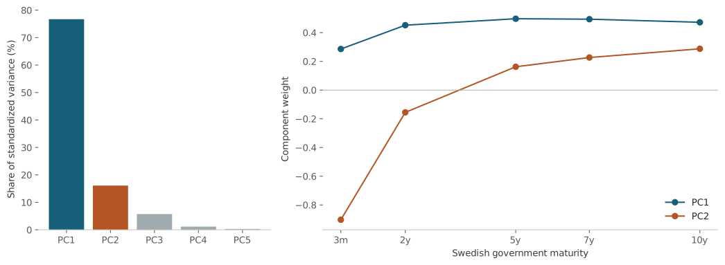
That percentage describes variation in the government yield curve. A single inflation surprise can move both level and slope, while several different shocks can produce similar shapes. The familiar “level, slope, curvature” labels describe these patterns without identifying their causes. Tao Wu, Federal Reserve Bank of San Francisco, Economic Letter, 6 June 2003
Separating expected policy from term premia requires a model of the yield curve. Measuring bank funding and retail pricing more directly requires bank data. PCA alone cannot recover those economic components.
A stronger extension would combine the Swedish announcement shocks with foreign policy surprises, bank-level funding information and matched-maturity SEK swaps. Use local projections or an instrumented system, separating current-rate, policy-path and term-premium news. The public Swedish event dataset and New York Fed ACM components are available inputs. This project has identified those datasets but has not fitted that structural extension. Swedish event data · US ACM data
Adding CPI, exchange rates, employment, bond yields and mortgage rates to one unrestricted regression would mix causes, mediators and responses. A claim such as “inflation drives X% and America drives Y%” would depend heavily on ordering, shock definitions and assumptions. No defensible causal percentage allocation is established here.
To interpret a changing mortgage quote, watch three domestic prices: the policy rate, the Swedish five-year government yield, and the gap between mortgage-bond and government yields. Together they represent short-rate pressure, the longer curve and additional funding costs.
The model asks what usually happened to mortgage rates when one of those prices moved and the others stayed unchanged. An actual announcement can move several at once, so the result describes part of a scenario.
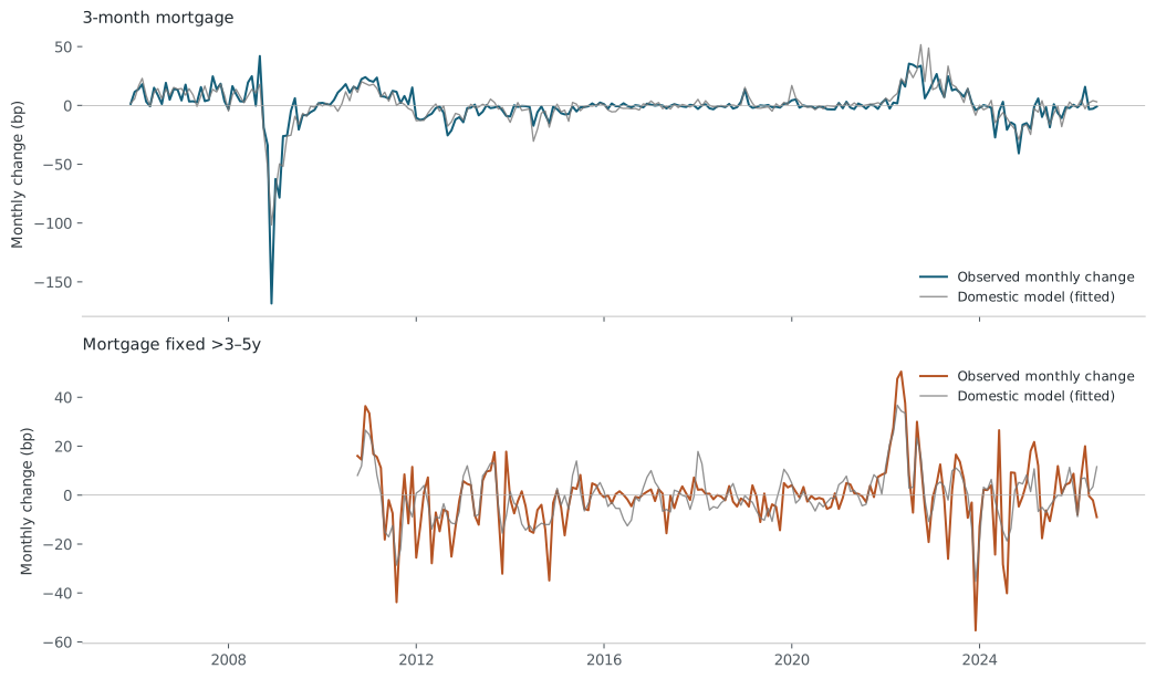
A bank may reprice over several months, so the equation allows each input to affect the mortgage in the current month and the following two. The coefficients are estimated separately for the 3-month and fixed >3–5-year mortgage series.
These three domestic prices describe the historical mortgage changes much better than US yields alone. Over the same 190 months, they account for about 74% of the variation in floating-rate changes and 57% in fixed-rate changes. The US-only model accounts for about 2% and 25%, respectively. This supports using domestic prices to interpret a bank’s repricing, even when the original news came from abroad.
These percentages measure fit to the history used for estimation. Forecasting needs a separate test against months the model had not yet seen.
| Inputs, each with lags 0–2 | 3-month mortgage R² | Fixed >3–5y mortgage R² |
|---|---|---|
| US only | 2.2% | 24.5% |
| Policy only | 68.7% | 2.6% |
| Domestic | 73.9% | 57.1% |
| Domestic + foreign | 75.2% | 58.5% |
Identical outcome months within and across columns. These percentages describe in-sample fit of changes, not shares of economic causation or forecast accuracy. Adding predictors generally increases in-sample R².
In the full available histories, the expanded foreign model’s US terms are jointly significant at the 5% level for fixed mortgages (p≈0.044), with a negative summed coefficient. They are not clearly significant for floating mortgages (p≈0.34). With overlapping predictors and different samples, this is insufficient evidence that a US tightening lowers Swedish mortgage rates.
Hold two inputs unchanged and vary the third. The model then traces a line between the assumed market change and the associated mortgage change. A steeper line means more of that input change reaches the fitted mortgage response. The shading shows how precisely the slope was estimated.
For example, using the full history, a one percentage-point rise in the Swedish five-year yield is associated with about 0.74 percentage points on a newly fixed mortgage and 0.17 on a three-month mortgage, with policy and the funding gap unchanged. The model adds that response over three monthly observations. If a new fixed offer began at 3.00%, adding 0.74 points would put the scenario at 3.74%. Your existing fixed contract would retain its agreed rate until expiry.
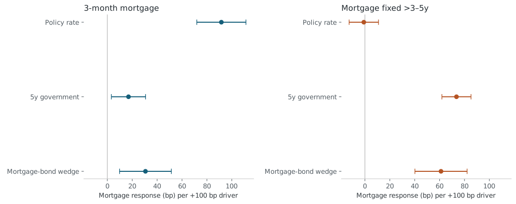
The policy line for fixed mortgages is close to flat in the full sample because this comparison holds the longer curve unchanged. A real Riksbank announcement can also move that curve, reaching fixed offers through a channel we have deliberately held still. Read each line as one part of a scenario, rather than the total effect of an announcement.
The historical period also changes the slope. Using only data since 2015 lowers the floating response to a one-point policy increase from about 0.92 to 0.75 points. The corresponding fixed response to a one-point government-yield increase rises from about 0.74 to 0.79 points. Try both samples before relying on a scenario; the gap between them is one indication of how much a simple model can depend on its history.
The Riksbank’s public STIBOR series ends in July 2020. A robustness model through June 2020 substitutes STIBOR for policy and obtains 87.9% in-sample fit for floating changes, with a cumulative STIBOR coefficient near 0.95. In that model, the extra five-year government coefficient is close to zero. This suggests the full-sample policy model’s longer-rate terms partly proxy omitted short funding conditions. The samples differ, so the R² change cannot be attributed solely to STIBOR.
The model uses new and renegotiated MFI agreements, avoiding the 2019 extension of the broader aggregate to nonbank mortgage companies. Changing bank and borrower composition remains possible. The >3–5-year bucket has a varying maturity mix. Monthly averaging blurs within-month announcement timing. The source observations and sample choices are retained with the underlying research.
We repeatedly estimate the model on earlier months and check its predictions against later outcomes. Market prices arrive sooner than SCB’s mortgage averages, so they can help estimate rates before publication. The benchmark simply keeps the latest published mortgage rate unchanged. We allow for publication delays but use revised historical data, which limits how closely this recreates forecasting at the time.
Every configuration is tested against the same 91 target months from January 2019 to July 2026. Start with the issue-month forecast below, then move to a later target. The chart shows both the actual rate and what each approach would have predicted; the smaller chart underneath shows when the model overestimated or underestimated it.
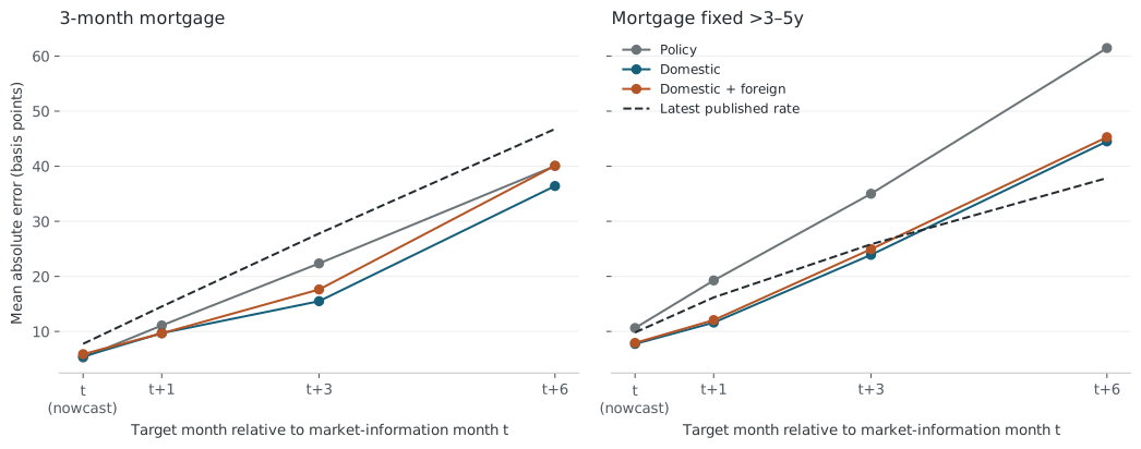
The model is most useful close to the date it is issued. For that month, it reduces the average floating-rate error from 14.5 to 9.7 basis points, and the fixed-rate error from 16.2 to 11.6 basis points. Ten basis points is one tenth of a percentage point, the difference between 3.00% and 3.10%. On SEK 5 million, that difference is about SEK 417 in monthly gross interest. An average error is not a bound: individual predictions can miss by considerably more.
Five months after issue, the fixed-rate model performs worse than keeping the last published rate. In quiet periods, predicting no change can also be hard to beat. Adding US and German yields does not consistently improve the forecasts.
Use the model to interpret the next offer and test a specified rate change against your budget. Its forecasting record provides little basis for predicting the average floating rate over a three- or five-year fix.
| Target relative to market-information month | 3-month: model / unchanged | Fixed >3–5y: model / unchanged |
|---|---|---|
| Latest unreported month t | 5.5 / 7.8 | 7.7 / 9.8 |
| Following month t+1 | 9.7 / 14.5 | 11.6 / 16.2 |
| Month t+3 | 15.5 / 27.8 | 23.9 / 25.8 |
| Month t+6 | 36.4 / 46.8 | 44.5 / 37.9 |
Entries are average absolute errors in basis points; smaller is better. Market-information month t ends immediately before the model is issued in t+1. The t+6 target is therefore five months after issue. The previous month’s mortgage observation is generally still unpublished: both the model and the unchanged-rate benchmark use the latest published rate, from t−1.
Each horizon is estimated separately with expanding-window ordinary least squares, at least 84 usable training observations. Inputs include the selected market changes at lags 0–2, the latest published mortgage change and the latest published mortgage-to-reference gap. Domestic/foreign models also use the five-year government-minus-policy slope. The reference is policy for floating and for the policy baseline; it is five-year mortgage-bond yield for fixed domestic/foreign models.
At information month t, training labels must have outcome dates no later than t−1. There is no random train/test split. The underlying research retains detailed predictions, training cutoffs and results by period. The forecast publication month is recorded separately from the market-information month.
This is a revised-vintage historical backtest, not a reconstruction of every release as originally seen. SCB’s notes flag an October 2025 revision affecting 2022–2024 new-agreement rates. Release availability is approximated at monthly frequency; an operational daily model would need the actual release calendar and data vintages. Model forms were chosen on economic grounds during this research, not preregistered in an untouched experiment. No formal test of forecast superiority or calibrated future prediction interval is claimed.
Start with the rate you are offered, the years it covers and the share of the loan you want to fix. Compare that period with how long you may keep the home. Fixing protects the agreed rate on that portion of the debt. The certainty can be worth paying for even when you expect floating to cost less.
Compare a three-year fixed offer with the average floating rate you would pay across those three years. Include all the interest paid along the way; the rate at the end cannot tell you the total cost. A one-year fix gives one year of certainty; the next offer is unknown. To compare it with a five-year fix, both need the same five-year accounting window and an explicit assumption for years two to five.
For example, a 3.50% fixed quote against a constant 3.00% floating rate costs an extra SEK 2,083 a month on SEK 5 million, or SEK 125,000 over five years without amortization. If floating instead averages above 3.50%, the fixed offer saves interest. The quote already includes the bank’s price for fixing; the calculation compares the resulting payments.
A 1 percentage-point rise adds SEK 833 a month per SEK 1 million still on a resetting rate. Fixing half the loan halves that immediate exposure while the fix lasts. Set a tolerable increase alongside your cash reserve, amortization and BRF costs. A fixed rate stabilizes interest on the fixed portion; the whole housing bill can still change.
A longer fix protects more reset dates. A shorter one restores flexibility sooner. If you stagger terms, less debt resets at once, but moving the loan to another bank can become harder. Compare the extra cost with the years of certainty you receive, especially years when your budget may be tight.
Rate certainty, fixation periods and the trade-off when splitting maturities: Konsumenternas: Boränta.
If you sell or change lenders before the fixed period ends, early-repayment compensation (ränteskillnadsersättning) can change the result. Keeping the loan and substituting the new home as security may be possible, but needs the lender’s approval. Konsumenternas advises avoiding a fixation longer than the time you expect to keep the home. Fixation and intended holding period · Early repayment and security substitution
Rising SEK swaps and mortgage-bond yields can make the next fixed offer worse before your 3-month rate changes. Waiting can therefore change the price of certainty. Whether fixing costs less over several years still depends on the rates you would otherwise pay. A changing policy path is more relevant to future floating resets. Its effect is already partly reflected in fixed offers, so an expected Riksbank cut is not by itself a reason to stay floating.
The model’s short forecasting horizon cannot validate the one-to-five-year paths above or assign them probabilities. Compare several paths with actual offers and your budget to judge how much certainty you want to buy.
When collecting quotes, record the negotiated rate, fixation length, fees, offer validity, start date, discount expiry and repayment terms. An indicative quote can change before the loan starts unless separately locked. Konsumenternas: comparing and locking rates. Consumer-rule references checked 9 September 2026.
The most dependable calculation is the cash consequence of a specified mortgage rate. Each extra percentage point costs SEK 833 per month per SEK 1 million borrowed, before tax effects. At SEK 5 million, that is SEK 4,167 per month. A two-point rise doubles the increase. This arithmetic does not require successfully forecasting the rate.
The scenario tool applies the research coefficients to a new or resetting mortgage and converts the result into gross interest. A driver shock is held constant in level after its initial move; the fitted response accumulates across three monthly observations. Other model inputs are held fixed. Values can be changed directly to test larger affordability stresses.
Default loan and stresses are illustrative. The starting 2.74% floating / 3.27% fixed values are rounded July 2026 MFI averages, not personal offers. Existing fixed loans retain their agreed rate until repricing. Calculations exclude principal repayment, taxes, fees and household income changes.
An association’s debt can raise future fees when its loans refinance. As a rough allocation, multiply debt per square metre by the apartment’s area, the share repricing and the assumed rate change. This estimates the extra interest attributable to that area. Actual fee decisions depend on the association’s budget, reserves, allocation rules and other income; a fee increase is not automatic.
Illustrative extra BRF interest allocated to this apartment: per month.
The July 2026 average was 2.74% for new and renegotiated three-month mortgages and 3.27% for mortgages fixed for over three to five years. Those averages cover different borrowers and contracts. They give market context, but comparing the offers available to you requires your own quotes.
| Observation | Rate | Observation date |
|---|---|---|
| Riksbank policy | 1.75% | 2026-09-08 |
| Swedish government 5y | 2.825% | 2026-09-07 |
| Swedish mortgage bond 5y | 3.259% | 2026-09-07 |
| Swedish government 10y | 3.101% | 2026-09-07 |
| US government 10y | 4.782% | 2026-09-07 |
| MFI actual 3-month mortgage | 2.74% | July 2026 |
| MFI actual fixed >3–5y mortgage | 3.27% | July 2026 |
Latest recorded market observations in the Riksbank API as retrieved 8 September; these are not live executable prices. July mortgage averages were released in August. Market series · SCB July release
Higher interest rates can increase your payments while reducing what the next buyer will pay. If that lowers the sale price, leaving an uncomfortable mortgage can become harder just when you want to move.
A buyer compares the services a home provides with the cost of owning it. Higher expected borrowing costs reduce what that buyer is willing to pay, other things equal. A rise expected to persist has a larger effect than a brief spike. The Riksbank’s housing-cost analysis describes this mechanism, alongside buyers postponing a purchase or choosing a smaller home when their monthly budget tightens. House prices and interest-rate expectations, pp. 3–10
The lender can impose another limit. Swedish banks assess whether income covers stressed interest costs, principal repayments, housing expenses and living costs. Tighter assumptions can reduce the approved loan, although banks’ stress rates do not follow mortgage quotes one for one. Buyers’ incomes, available homes and expectations also change. These channels explain why rates can weaken demand; they do not establish a stable percentage fall in prices for each percentage-point rise in rates. Riksbank: how mortgage credit is assessed
The exit can become slower as well as less profitable. In the 2022–23 downturn, the Riksbank recorded falling prices and fewer sales despite a relatively large stock of homes for sale. It warned that lower prices could leave owners staying longer than intended or owing debt after selling. Inflation and interest costs rose together in that episode, so it is not a clean estimate of the effect of rates alone. Financial Stability Report 2023:1, pp. 39–41
Consider a SEK 5 million home financed with SEK 4 million of debt. You start with SEK 1 million of equity. A 10% price fall removes SEK 500,000: half your equity, although the home lost only a tenth of its value. At a 20% fall, its value just equals the debt. Selling costs would then require additional cash. These are balance-sheet calculations with unchanged debt, before fees and taxes; a price fall alone does not make a payment default inevitable.
Suppose the SEK 5 million home falls to SEK 4 million, then later returns to SEK 5 million. If you can keep the home and meet its costs, you still own the asset when its value recovers. If a cash shortage leads you to sell at the low point, a later recovery in that home’s price no longer restores your equity. This hypothetical recovery helps only while you still own the home. The intervening cash shortage and sale change your outcome.
A fixed rate can protect monthly headroom during its term. That may give you time to wait for a buyer or avoid selling into a weak market. It does not protect the resale price, your income or the association’s fees, and leaving the loan early can add a cost. If the fixed quote costs more initially, that extra payment also uses some of the cash you could otherwise save. Use the offer comparison to price the protection, then test the resulting budget here.
Before buying, test a period on one income, higher association fees or a move sooner than planned. Consider the loan size, cash reserve and fixed-rate period together. Lower debt reduces payment exposure and leaves room for a larger price fall before equity disappears. A reserve can pay the bills while you wait; using the equity in your home requires a sale or further borrowing. Choose a payment plan you can maintain through those periods.